|
Generating
Outline Coordinates
|
|
CartesianDiatom-EFA imports outline coordinate data from files generated by tpsDIG and ImageJ software in a variety of formats. It also accepts data which are entered by cut/paste transfer and by typing directly into Excel. Four Orientation Landmark x,y-coordinates are expected to preceed the coordinate data for an outline in the file, but these can be by-passed. The accepted formats and procedures for generating them are explained below; sample data files are provided in the testdata folder as part of downloading the program. Custom formats can also be designed by CartesianDiatom. |
|
Orientation
Landmarks |
||
| tpsDIG2 ImageJ custom cut/paste or direct entry |
 |
|
|
To digitize image outlines
using tpsDIG2, |
|
1 Place image files and micrometer image in the same directory. The micrometer image should be the first image in the directory. tpsUtil will alphabetize the files by their names as they are loaded, so consider adding a prefix to the micrometer image filename to make it first in the list, such as "A1Micrometer", or use the options available in the tpsUtil setup to reorder the files. Alternatively, this tps file can be constructed without tpsUtil; see tpsDIG2 Help, p. 9 (pdf p. 13) 2 Open tpsUtil. [Operation Frame] Select Build tps file from images. 3 [Input directory Frame] Select Input. Locate the image file directory and select any one image in it. Select OPEN. The name of the directory of files to be imported is indicated in the Input directory frame. 4 [Output file Frame] Select Output. Enter a name of your choice for the file. Leave the file extension as *.tps. Select SAVE. This extension is required for the file to be imported by tpsDIG. The path and name of the file-to-be-created are indicated in the Output file frame. Note the file will be placed in the same directory as the images. This is a tpsDIG requirement. 5 [Actions
Frame] Select SetUp. A "Build tps file" window
appears listing on the left all images potentially to be included in
the new *.tps file. On the right are operations controlling the selection
of these images. Initially all images are selected to be included, as
indicated by the checks in the boxes to the left of their file names.
If all images are to be used, Select Include all, then
Create. 6 In the remaining tpsUtil window, select Close. The newly created file is ready for use by tpsDIG2. |
|
tpsDIG2 1 Images should be in a *.tps file format. The micrometer image should be first image the file. See tpsUtil if this is not the case or the tpsDIG2 documentation.
2 Open tpsDIG2. Select File | Input Source. Choose
the *.tps File containing images for processing. Then select
Open. 3
Calibrate the system using the stage micrometer image. Select Image
Tools | Measure. Enter a reference length and then make two clicks
on the micrometer spanning that length (1st click - release (do not drag)
- 2nd click). Select OK. Save this calibration by selecting
from the Main Menu File | Save data . Save in the same tps file
displayed in the filename window and finally choose Overwrite. 4
Select the next image (first outline image) by using the right-pointing
red arrow at the left end of the Main Menu. You may need to make a magnification
adjustment and scroll the window to center the specimen-of-interest. |
||
|
5 Digitize the 4 Orientation Landmarks using
the Digitize Landmarks Tool.
Choose the Tool by clicking on
its icon (it looks like cross-hairs) or selecting it from the menu Mode
from the Mode | Digitize Landmarks. The markers can be repositioned
by switching to Edit mode. |
LM=0 |
|
|
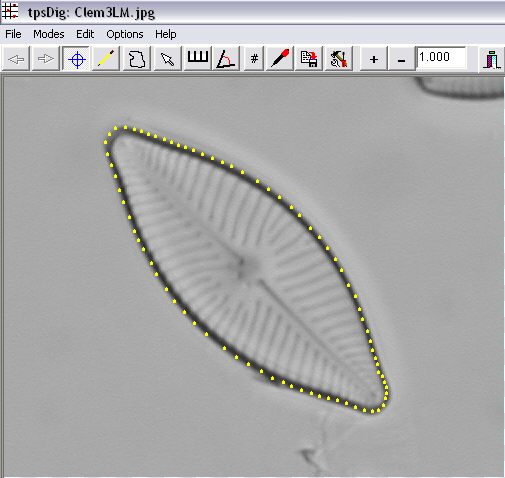
6 Choose ONE
the following modes of digitizing the outline: Landmarks
Tool, Curves Tool, or Outlines
Tool. See tpsDIG2 Help documentation
for details on the use of these tools. |
||
|
Digitize Landmarks
Tool The
outline coordinates will be recorded in the data file immediately following
the 4th Orientation Landmark's coordinates. On the right they are highlighted
in green. The "LM=74" in line 4 of the data file indicates there
are for this outline 74 points recorded: 4 orientation landmarks (blue)
and 70 outline (green, only 6 are shown). Sample
data files of 3 outlines using the Landmark Tool are provided: PclemLM.tps
(with Orientation Landmarks), PclemLM_NoOL.tps (without Orientation Landmarks). |
LM=0 IMAGE=C:\cdi\clem5\Olympus100X1.8x.JPG ID=0 LM=74 1090.00000 1203.00000 939.00000 333.00000 1074.00000 755.00000 1022.00000 762.00000 1092.00000 1208.00000 1114.00000 1198.00000 1128.00000 1177.00000 1135.00000 1158.00000 ... 1059.00000 1198.00000 1076.00000 1208.00000 IMAGE=C:\cdi\clem5\P1270001.JPG ID=1 SCALE=0.022667 COMMENT=comment VARIABLES=A5 ... |
|
|
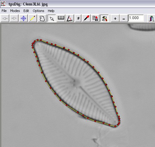
Other infomation about the outline will follow these data as indicated by tpsDIG keywords: IMAGE (required), ID (required) , SCALE, COMMENT and VARIABLES. Sample data files for 3 outlines using the Curves Tool are provided : PclemCU.tps (with Orientation Landmarks), PclemCU_NoOL.tps (without Orientation Landmarks). |
|
LM=0 IMAGE=C:\cdi\clem5\Olympus100X1.8x.JPG ID=0 LM=4 1090.00000 1203.00000 939.00000 333.00000 1074.00000 755.00000 1022.00000 762.00000 CURVES=1 POINTS=75 1092.00000 1208.00000 1114.00000 1198.00000 1128.00000 1177.00000 1135.00000 1158.00000 ... 1059.00000 1198.00000 1076.00000 1208.00000 IMAGE=C:\cdi\clem5\P1270001.JPG ID=101 SCALE=0.022667 COMMENT=comment VARIABLES=A5 |
|
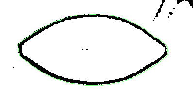
[Note: I have found the following Outline Tool instructions work in tpsDIG (version 1), but not in tpsDIG2, version 2.01, in that the file saving routine is incorrect. However, they do work in the current version of tpsDIG2, version 2.12, downloaded 9 July 2009. When in-between things changed I do not know. ... rke 9 July 2009.] This is easily the
most complex of the 3 options. Select
Outlines. In the Object Frame select the "light"
button. Restore returns the original non-binary image, that is, either color or grayscale image. Use it when you think you need to start your thresholding from the beginning. After securing a satisfactory binary image, select Modes | Outline Mode (or select the Outlines icon). The cursor changes to an open outline with an arrow tip. Select a point near but to the right of the outline* and click the left mouse button (the arrow tip indicates the point). A colored (yellow or green) line is drawn around the contour. Right click the image and a pop-up menu will appear; select Save as XY coords. The number of coordinates in the outline appears in a "No. of coords." window. Select OK. *
Once you click the cursor to start the outline, the program searches horizontally
to the left until it finds the junction between the black and white pixels,
and then it follows that interface (= outline) recording all the pixels
at the interface. Do not click on the outline directly to start the automatic
outlining, slightly to the right of where you want the recording
of coordinates to start. You also should investigate the difference between
the "dark" and "light" options on the Image Tools
| Outlines form as to where the tracing of the outline occurs. Further details and variations on the above can be found in tpDig2 Help. Other infomation about the outline will follow these data as indicated by tpsDIG keywords: IMAGE (required), ID (required), SCALE, COMMENT or VARIABLE. Sample
data files using the Outline Tool are provided: PclemOU.tps (with Orientation
Landmarks), PclemOU_NoOL.tps (without Orientation Landmarks). |
|
LM=0 IMAGE=C:\cdi\clem5\Olympus100X1.8x.JPG ID=0 LM=4 1090.00000 1203.00000 939.00000 333.00000 1074.00000 755.00000 1022.00000 762.00000 OUTLINES=1 POINTS=1564 1092.00000 1208.00000 1114.00000 1198.00000 1128.00000 1177.00000 1135.00000 1158.00000 ... 1059.00000 1198.00000 1076.00000 1208.00000 IMAGE=C:\cdi\clem5\P1270001.JPG ID=101 SCALE=0.022667 COMMENT=comment VARIABLES=A5 |
|
|
||
|
|
||
|
For ImageJ we
describe two ways in which the outline can be digitized: The protocol for each consists of 9 steps; only step 7 differs between the two. |
| 1 |
IMAGE FOLDER SETUP |
|
| 2 |
OPEN ImageJ. |
|
| 3 |
IMPORT IMAGES |
|
| 4 | CALIBRATE
the system using the Set Scale option and the stage micrometer image.
If you do not calibrate the system your results will in pixels. |
|
| 5 | SELECT
A VALVE (SPECIMEN) |
|
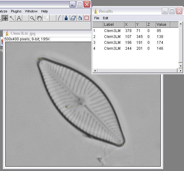
| 6 |
If
you hold the Shift key down while you click, the marked yellow
points will remain on the screen; if you do not, only the most recent
one is displayed. This does not affect their being written to the Results
window, only their display. If
you choose not to digitize the 4 Orientation Landmarks, then just skip
this section but remember to uncheck the Orientation
Landmarks box during the Import Outlines process. |
|
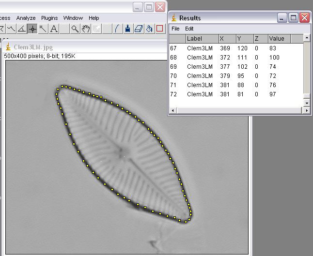
| 7 | OUTLINE
THE VALVE. Continue using the Crosshair Tool to digitize the valve outline by clicking on points which well-represent its curvature; for each point a line of data will be written to the Results window and a yellow marker placed on the image. |
|
|
Suggestions for digitizing: - Digitize
clockwise; although this is not necessary, it will reduce processing time
in the EFA. However, regardless of the direction, do not make the last
point chosen either the same as or beyond the starting point. |
||
| 8 |
SAVE DATA
- Orientation Landmarks and Outline Coordinates |
|
| 9 |
NEXT VALVE or EXIT? Select the next valve
to be analyzed (Return to Step 6), or, if your sesssion is done,
make sure you have made the last Save As of your Results Window.
|
|
| WandAuto Tool |
| 1 | IMAGE FOLDER
SETUP Place all outline images in the same folder along with the image of the stage micrometer used for calibration. |
| 2 | OPEN ImageJ. Check two initial settings of the program: (1) Select Analyze | Set Measurements | Check the box to "Invert Y-coordinates". That is, Y-coordinates should be inverted. (2) Select Edit | Options | Colors. Set the Foreground to "white", Background to "black", and Selection to "yellow". |
| 3 | IMPORT
IMAGES Select File | Import | Image Sequence. Choose a single file from the folder with the images, then select OPEN. Check the box to "Convert to 8-bit Grayscale" in the "Sequence Options" window which opens. Leave the other settings as they are. Select OK. |
| 4 | CALIBRATE
the system using the Set Scale option and the stage micrometer image. |
| 5 | SELECT A
VALVE (SPECIMEN) |
| 6 |
If
you choose not to digitize the 4 Orientation Landmarks, then just skip
this section
but remeber to uncheck the Orientation
Landmarks box during the Import Outlines process. |
| 7a |
Select
Image | Adjust | Threshold. The image window will
preview a binary image of the outline and a new "Threshold"
window will pop-up.
The histogram: The histogram at the top of the window is a frequency
distribution of the grayscale values of all the pixels in your image.
The grayscale values values are scaled on the horizontal axis from 0 (pure
black) to 255 (pure white). Color: There are 3 options in the color window: red, black-and-white, and over/under. The default is red. Change the color setting to "Over/Under". Pixels with grayscaled values less the minimum are blue, those with grayscale values greater than the maximum threshold are green and all pixels between the two thresholds are black. Use the scroll bars to investigate the relationship between the threshold settings and the distribution of colors in the image - paying particular attention to the distribution of black. Change the color setting to red. The image now consists a sets of colors with red representing the pixels with grayscale values between the two thresholds. For an image with the same thresholds, red in this color pattern corresponds to black in the "over/under" mode. In "black/white" mode, the area between the thresholds is represented as black and pixels below the minimum threshold AND above the maximum are white. Take a few minutes and explore the effects of moving the scroll bars on the outline and of viewing the effects using the 3 different color modes. Where is the outline of the valve wall? You will have noticed in your exploration of the threshold window that as you changed threshold maximima and minima that the breadth of the image sector corresponding to the between-threshold area changed. Somewhere in that area should be the outline you are after. We cannot provide specific instructions on how to secure that outline as it will depend on many factors of which we cannot be aware, e.g. the structure of the mantle wall of your diatom, the focus of your image on the mantle wall, etc.
As a first approximation to the outline we want to capture, let us assume
in most diatoms that the darkest area of the image in the region of the
wall will coincide with the mantle wall (outline), then we might try to
only display only relatively "dark" pixels, those with brightness
values toward the left end of the histogram. For use of the WandAuto (or
Wand) tool we need the thresholded outline we use is (1) continuous, and
(2) smooth on its exterior margin. When the contour of the outline is
captured, we aim to capture the coordinates of the black pixels which
form the outer border of its outline. What goes inside that border does
not concern us in this process. |
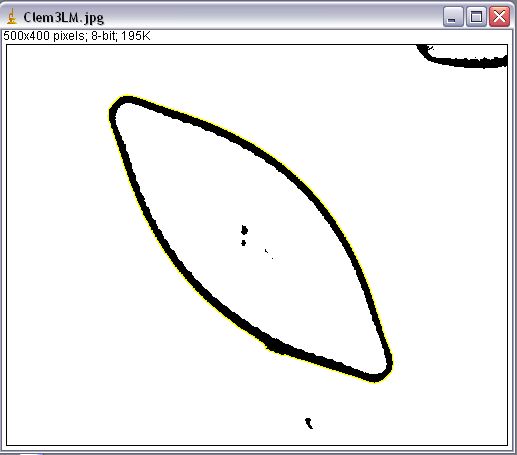
| 7b |
OUTLINE THE VALVE. The default Wand Tool in ImageJ's main menu can be used to capture the outline automatically, but it does not by itself record the coordinates of the outline anywhere without a set of additional commands. However, there is a tool in ImageJ which both captures the outline and writes the x,y-coordinates of the outline to the Results window. To load this tool for use: From the main menu,
choose Plugins | macros | Install. From the macros directory
select the tools folder and open it. Finally select the file named
WandAutoMeasure. and Open it. A small green wand icon will
appear in the menu which accesses this WandAuto tool; it typically loads
about 2 menu items to the right of the conventional Wand tool. Upon completion of the trace of the outline, the pixel of all coordinates in that trace will be written to the Results window; there may be several thousand of them. If the selection made by the WandAuto Tool does not get all (and more-or-less only) black pixels on the exterior outline of the valve, the trace is not acceptable and needs to be re-done. The outline will be highlighted in yellow (or red). To turn the AutoWand Tool's outlining off, that is, to deselect the outline, so that you can use it again on the same specimen, choose Edit | Selection | Select None. The trace of the outline made by the Wand and WandAutoMeasure Tools in ImageJ captures the coordinates of the first point as also the last point, that is, the first point is duplicated in closing the trace. For EFA this last duplicated point is removed when the data file is processed by CartesianDiatom-EFA. Capturing an outline
which is satisfactory for EFA is often not a simple task. You will probably
need to explore development of a scheme based on the above for your own
specimens. ImageJ provides a vaiety of additional options. |
| 8 |
SAVE DATA - the Orientation
Landmarks and the Outline Coordinates These
data are all in the Results window at this stage. |
| 9 |
NEXT VALVE or EXIT? Select
the next valve to be analyzed (Return to Step 6), or, if your sesssion
is done, make sure you have made the last save of your Results
window. |
 Select
Process | Binary | Threshold.
Select
Process | Binary | Threshold.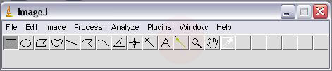
|
The custom option is designed for special importing routines CartesianDiatom has designed for specific users. Each requires a code to run and will be of no interest unless a protocol has been specifically designed for you. |
|
Enter data directly onto the
OrigOutline worksheet conforming to its expected
structure. |
|
The following sample data files have been included in the /testdata/ folder as part of the program download: PclemLM.tps - tpsDIG2
generated; 3 outlines with Orientation Landmarks using the Landmark Tool PclemCU.tps - tpsDIG2
generated; 3 outlines with Orientation landmarks using the Curves Tool PclemOU.tps - tpsDIG2
generated; 3 outlines with Orientation Landmarks using the Outline Tool ijPclemC - ImageJ generated;
3 outlines with Orientation Landmarks using the Crosshair (= Point) Tool |
Updated 7 July 2009
 This work is licensed under a Creative Commons Attribution-Noncommercial-No Derivative Works 3.0 United States License. |